Jiarui Wang (Project Researcher, Department of Earth and Planetary Science)

Yusuke Miura (Associate Professor, Department of Earth and Planetary Science)

Makoto Koike, Associate Professor, Department of Earth and Planetary Science

Key points of the presentation

• By devising the expression of the gas-liquid boundary ^(Note2) in the embedded boundary method ^{(Note 1)}, we have developed a method to simultaneously and accurately numerically calculate (simulate) the flow of water and surrounding air inside a falling raindrop of 0.5 mm or less in diameter.
• Although the application of the new method is limited to raindrops of 0.5 mm or less in diameter, it is important to note that it can now estimate the velocity of falling raindrops in a variety of environments where experiments are difficult.
• We showed that the empirical equation for the atmospheric pressure and temperature dependence of raindrop fall velocity used by weather and climate models has an error of up to 10%, and proposed a more accurate empirical equation.

Summary of Presentation

In weather and climate models that use supercomputers such as Fugaku to predict weather and climate, not only rainfall but also global warming can change depending on how the falling velocity of precipitation particles is set. However, until now there has been no method for accurately estimating fall velocity, and empirical equations based on experimental data from the 1940s to 1960s were used for raindrops. However, the reliability of the empirical formulas has not been verified under atmospheric conditions that differ greatly from those in the laboratory.

Project Associate Researcher Jiarui Wang, Associate Professor Yusuke Miura, and Associate Professor Makoto Koike of the Graduate School of Science, The University of Tokyo, have developed a method to accurately calculate the falling velocity of deforming raindrops with a diameter of 0.5 mm or less (Figures 1 and 2).

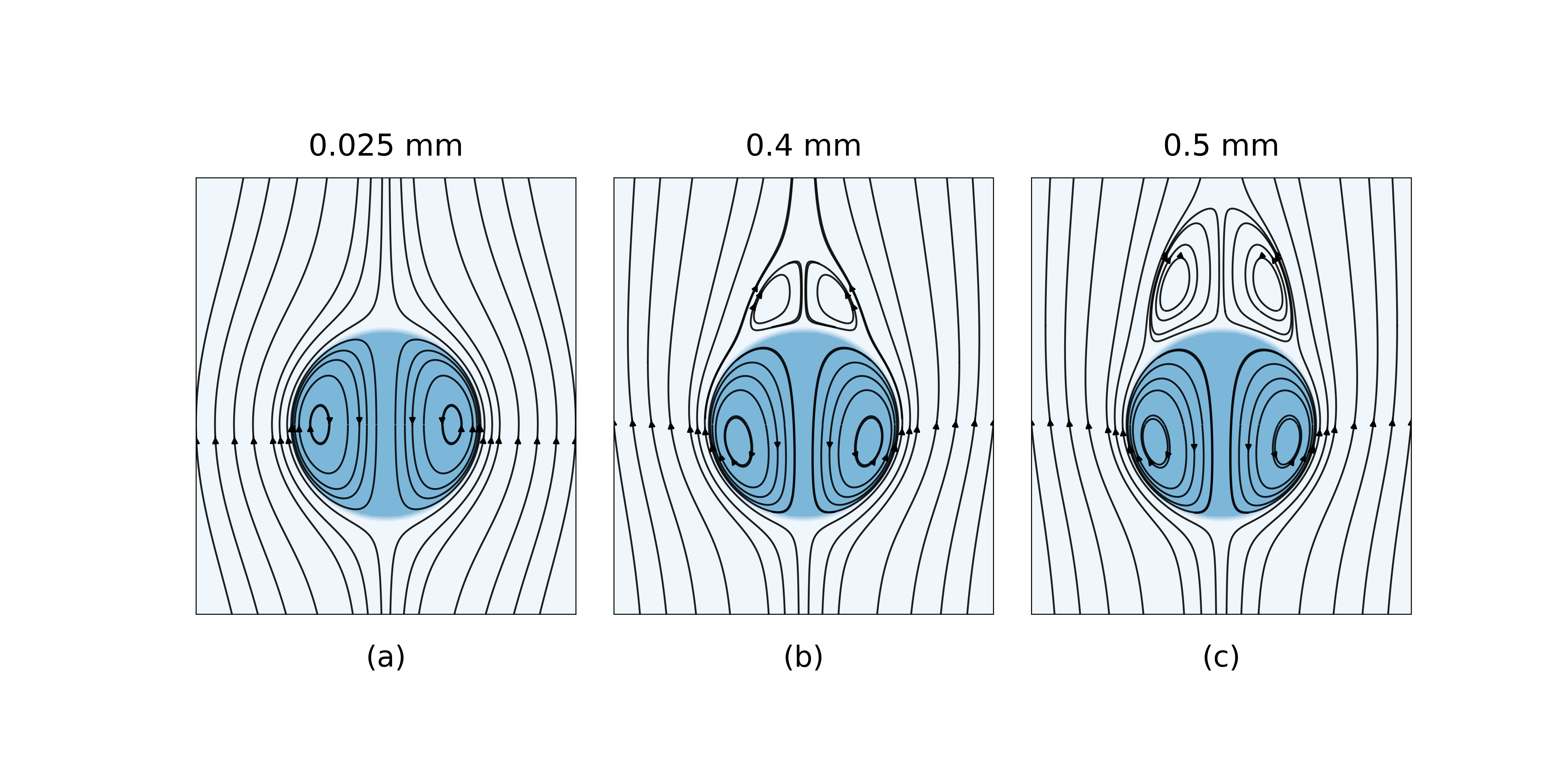
Figure 1: Water and air flow (streamlines) inside and outside falling raindrops of 0.025 mm, 0.4 mm, and 0.5 mm in diameter (shown in dark blue). When the diameter is small, the air flow simply wraps around the raindrop, but as the diameter increases, the flow becomes more complex and vortexes are created above the raindrop.

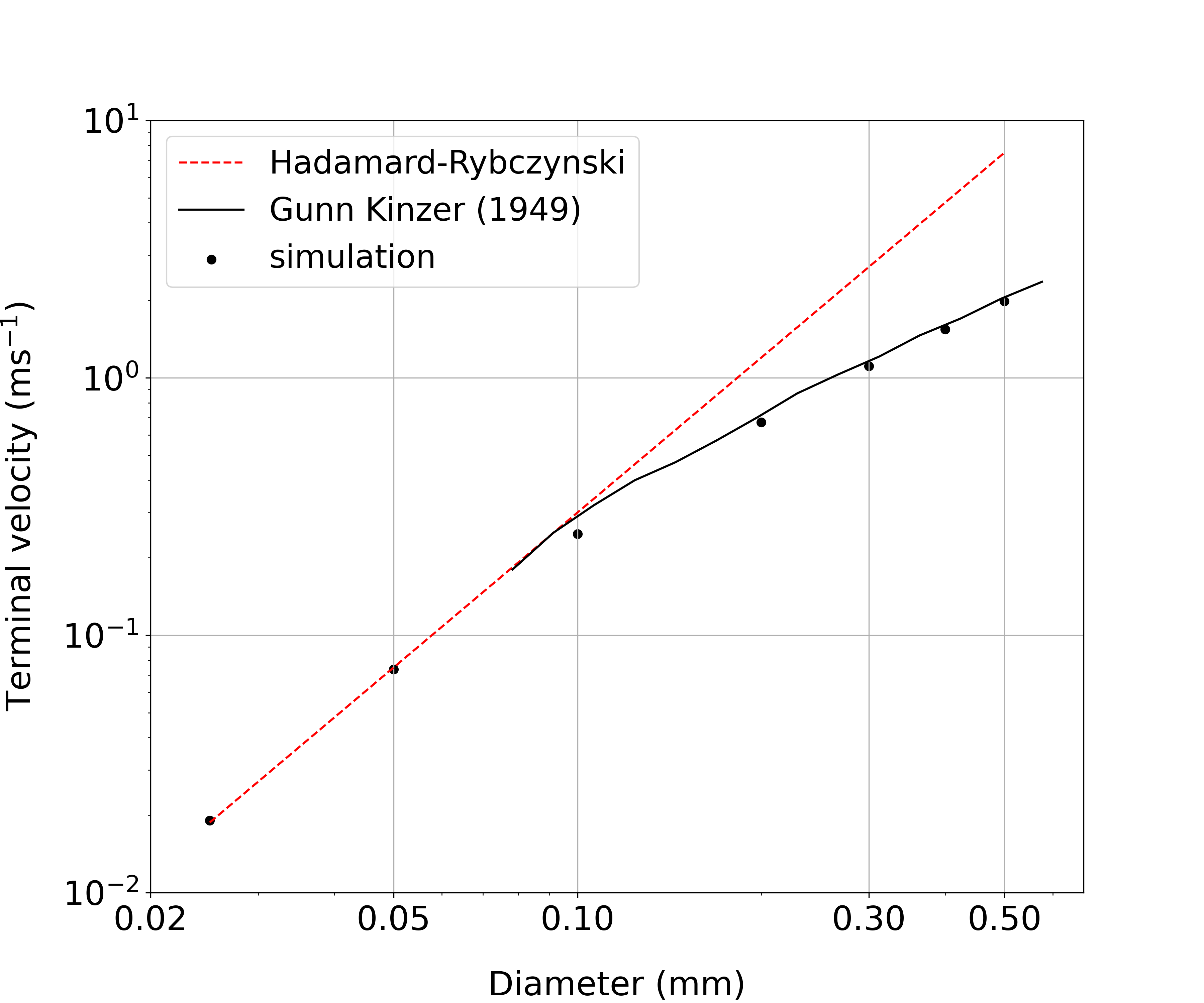
Figure 2: Relationship between raindrop diameter (horizontal axis) and terminal velocity of raindrop fall (vertical axis). The black dots represent the results of numerical simulations in this study, the red dashed line represents the Hadamard-Rybczynski asymptotic solution for small spherical cloud particles, and the black line represents the experimental data by Gunn and Kinzer (1949).

In this study, a discrete delta function that preserves the structure of non-rotation was introduced into the representation of the gas-liquid boundary surface in the embedded boundary method, solving the problem of false (fake) flows that has been a problem with conventional methods. With this new method, raindrop fall velocity can now be accurately estimated for various atmospheric pressures and temperatures that have not been tested before, and the results show that the empirical formula for raindrop fall velocity has an error of up to 10 % (Figure 3).

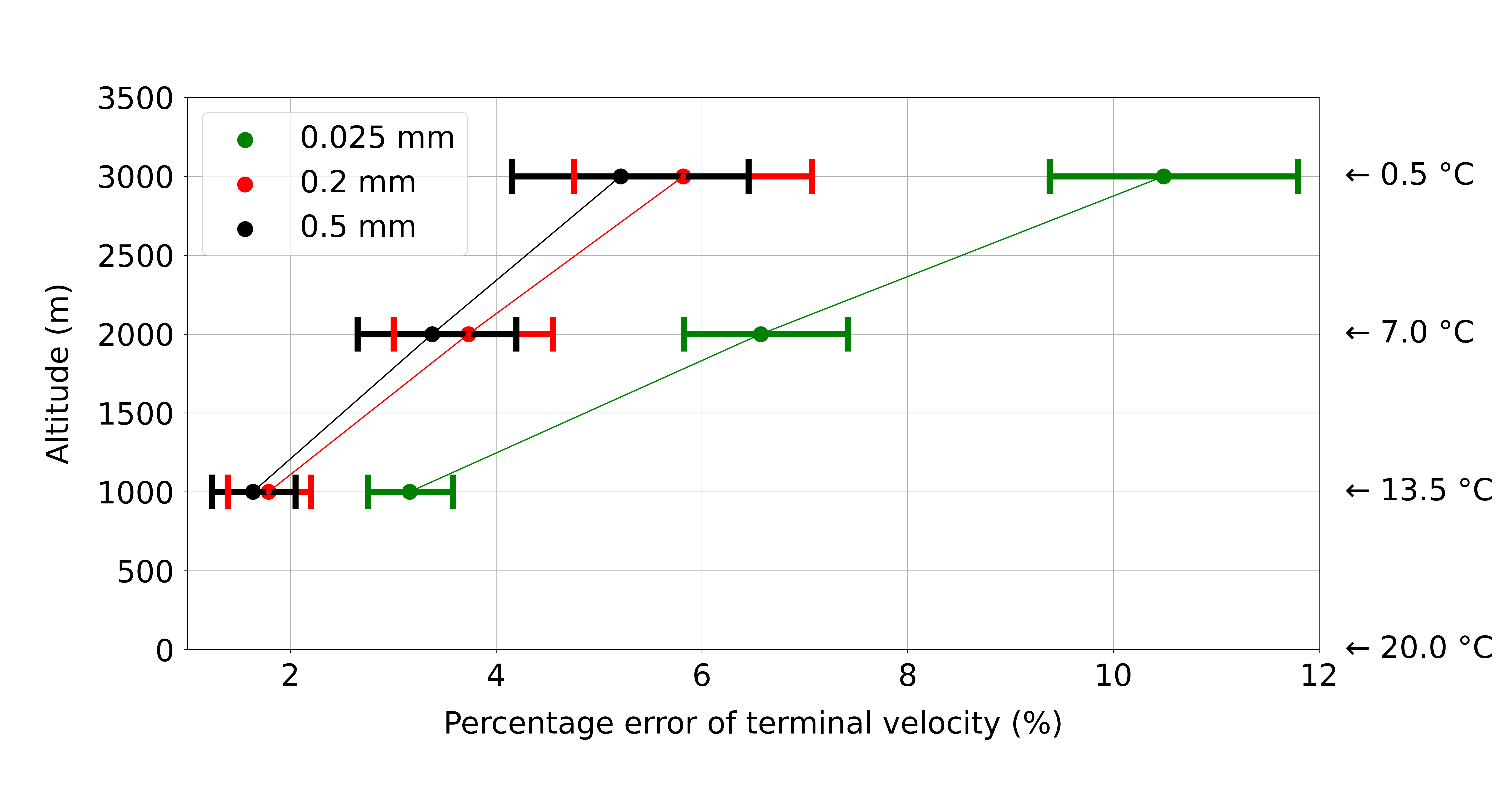
Figure 3: Errors in the calculation of terminal velocity using the currently used empirical formula, estimated at an altitude of 1000 m (air temperature: 13.5°C), 2000 m (air temperature: 7°C), and 3000 m (air temperature: 0.5°C). The altitude and temperature conditions are shown on the left and right of the vertical axis. The horizontal axis is the percentage of error.

Although this study was limited to raindrops of about 0.5 mm or less in diameter, it is important to note that it demonstrated the effectiveness of using numerical calculations (simulations) to estimate the falling velocity of raindrops that fall while being deformed. This research greatly improves the reliability of the equations used by weather and climate models to describe physical processes, and is expected to help reduce uncertainty in weather and climate forecasts.

Presentation Details

Background of Research
Large-scale numerical calculations (simulations) using weather or climate models are used in daily weather forecasts and predictions of future global warming. In weather and climate models, equations such as fluid dynamics, thermodynamics, and atmospheric radiology are expressed using various levels of approximation, and future weather and climate are calculated by integrating over time from appropriate initial values. The reliability of the results of these calculations depends largely on the reliability of the approximations, but there is still a high degree of uncertainty. For example, while atmospheric and oceanic currents can be calculated with high accuracy, the representation of cloud growth and decay has large uncertainties, which is a bottleneck in improving the reliability of climate predictions.

The cloud representation in climate models is becoming more sophisticated as supercomputers such as the Earth Simulator, the K computer, and Fugaku become faster and faster, and the time is approaching when we will be able to use equations that directly represent microscopic processes in clouds (cloud microphysical processes). In cloud microphysical processes, water in liquid and solid phases is divided into cloud water, raindrops, cloud ice, snow, and hail according to their sizes, and the changes in their abundance and number of particles over time are expressed in equations for calculation.

However, even when cloud microphysical processes are calculated, uncertainties about clouds remain. For example, for relatively large particles such as raindrops, it is necessary to set the falling velocity to represent precipitation. On the other hand, recent developments in numerical fluid dynamics have made it possible to calculate gas-liquid two-phase flows consisting of gas and liquid, and it has been expected that direct numerical simulation of raindrop fall in the atmosphere will become possible. However, the large density difference between air and water has hindered the calculation of the flow including the deformation of raindrops.

Details of Research
Project Researcher Jiarui Wang and his colleagues at the Graduate School of Science, The University of Tokyo, have developed a method to directly calculate the flow of water inside raindrops and the flow of air around raindrops simultaneously using the embedded boundary method (Figure 1). The conventional method has the problem of generating a false flow near the surface of raindrops in numerical calculations. Project Researcher Wang and his colleagues theoretically showed that the cause of this problem is a false rotation of the surface tension expressed using an isotropic discrete delta function. They then solved the false flow problem by using an anisotropic discrete delta function that preserves the structure of the non-rotation.

We validated the numerical simulation of raindrop fall by the embedded boundary method obtained in this study using experimental data from the 1940s-1960s and asymptotic solutions for the terminal velocity of spherical raindrop fall, which have been obtained under limited conditions, as reference values. For example, for raindrops with diameters of 0.025 mm and 0.05 mm, the results are in close agreement with the asymptotic solution of Hadamard-Rybczynski (a good approximation for raindrops smaller than 0.05 mm), and for raindrops with diameters of 0.1 mm, 0.2 mm, 0.3 mm, 0.4 mm, and 0.5 mm the results are in agreement with Gunn and Ginzer's (1949) experimental data (Figure 2). The data capture the slow increase in terminal velocity as the cloud particle diameter increases above 0.05 mm.

Four empirical equations for the atmospheric pressure and temperature dependence of raindrop velocity, which are widely used in weather and climate models, were tested for various atmospheric pressure and temperature conditions using the calculations of this method as reference values, and it was found that these empirical equations have large errors of up to 10 % (Figure 3). Although the errors are small for near-surface conditions, which are the reference for the empirical formulas, the errors become larger for altitudes of 1000 m (temperature: 13.5°C), 2000 m (temperature: 7°C), and 3000 m (temperature: 0.5°C), and so on, as one moves away from surface conditions. To reduce this error, we proposed a new empirical formula that can be used in weather and climate models.

Future Development and Social Significance
The embedded boundary method improved in this study assumes two-dimensional axisymmetry in the shape of raindrops and represents their fall in three-dimensional space. However, its application is limited to raindrops with a diameter of 0.5 mm or less. The reason for this is that raindrops with diameters larger than 0.5 mm exhibit non-axisymmetric motion when falling, and even larger raindrops exhibit chaotic motion. Further improvement of the method is needed to realize a realistic numerical simulation of raindrop fall, in which multiple raindrops grow by condensation, collision, and merging, and then disappear by breakup and evaporation. Currently, we are working on methods to represent raindrop collisions and mergers as well as raindrop surfaces in three dimensions.

The global cloud-resolving model, which is expected to be applied to climate prediction in the near future, will be able to represent cloud growth and decay more precisely by directly computing numerically the equations of cloud microphysical processes, and is expected to dramatically increase the reliability of physical processes that are essentially important for climate, such as cloud-radiation interactions. This research is aimed at understanding the cloud microphysical processes. This research will greatly improve the reliability of the empirical expression for one of the cloud microphysical processes. The results will not only improve the reproducibility of precipitation distribution and intensity, which are important for daily weather forecasting, but also provide a basis for improving the reliability of state-of-the-art climate prediction in the near future.

Journal

Journal name	Journal of the Atmospheric Sciences
Title of paper	The Terminal Velocity of Axisymmetric Cloud and Rain Drops Evaluated by the Immersed Boundary Method
Author(s)	Chia Rui Ong*, Hiroaki Miura, Makoto Koike
DOI Number	10.1175/JAS-D-20-0161.1
Abstract URL	https://journals.ametsoc.org/doi/10.1175/JAS-D-20-0161.1

Terminology

Note 1 Embedded boundary method

One of the methods in numerical fluid dynamics that can represent the boundary between two different materials, such as the atmosphere and water droplets. In general, fluid calculations use time-invariant points (grid points) and regions (inspection volume) that divide a three-dimensional space to calculate physical quantities, but the boundary between substances is represented as jagged. Therefore, a method was devised to express a deforming boundary by placing a marker at the boundary between two substances and tracking the motion of the marker. In the embedded boundary method, the Navier-Stokes equations, which are the dynamical equations of the fluid, are solved in the same way as in ordinary fluid calculations to reduce computational cost, while the boundary between the two substances is analyzed in a Lagrangian manner using markers. ↑up

Note 2 Gas-liquid boundary surface

The boundary surface between air and liquid (water). As shown in Note 1, the embedded boundary method tracks markers placed on the boundary surface and interpolates between markers by a function, making it possible to calculate the entire smooth boundary surface between air and liquid at each time. In this new method, various innovations, such as the marker relocation method, the composition of the smooth interpolation function, and the use of a discrete Heaviside function as the function representing the boundary, enable accurate computation while suppressing the computational cost. ↑up